The GPI Data Summary pages are for browsing through the 150 shots with stable conditions around the peak of the GPI puff, taken at the fastest framing rates, during the 2010 NSTX campaign. These shots are summarized in the table in GPI_2010_Top_Shots.htm.
Plots of average radial and poloidal velocities verses many of these plasma characteristics can be seen at gpivelplots.html.
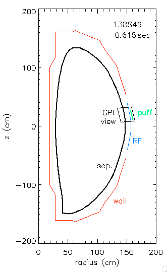
The image in the upper left of the GPI Data Summary page, just below "Click to play movie," is the last JPEG image used to create the associated QuickTime movie (accessible by clicking on the image). You may wish to right click on the image to bring up the movie in a new window. The view of the GPI diagnostic is a ~25 cm x 30 cm region just above the outer midplane of NSTX, where the radial direction is approximately horizontal and the vertical direction is approximately poloidal (i.e. perpendicular to the local radial and toroidal directions). The outward radial direction is to the right, and the ion diamagnetic and ion grad-B drift directions are downward. The magnetic separatrix (calculated from EFIT02) is shown by the solid white line. The vertical band of orange typically near the separatrix is from D-alpha emission. The projection of the RF antenna limiter is shown by the dotted line and the GPI gas manifold is shown by the vertical solid orange line just outside the RF antenna. This figure and QuickTime movies can be produced by fcplayer.pro, or cine2mpeg.pro (IDL routines that run on the PPPL Linux cluster) or blobmovies.html.
The second figure in the upper left shows "Blob Trails" +/- 1 millisecond around the peak of the GPI signal. The initial position of the blob is indicated with an ellipse representing a fit half way between the base and top of the blob. Only larger blobs are show. "MinHt>1.5" means the normalized height of the blob is 50% higher than the average. The separatrix (from EFIT02) is indicated by the line composed of long dashes. Different versions of this plot can be generated by blobtrails.html.
Validations of calculations of some blob tracking parameters have been made.
The "GPI Center Averages" figure shows the GPI emission averaged for each frame in a poloidal band +/- 10 pixels around the vertical center. This figure is smoothed in radius and highly smoothed in time (over ~1 msec). The location of the separatrix at the various times is shown by the dashed black line (usually) going from bottom to top. The two horizontal dashed black lines are 10 msec around the time of the peak of the smoothed GPI total trace. This figure can be produced by gpicont.pro. See GPIcompFit.html to see where LRDfit04 and EFIT02 fits place the separatrix for some of these shots.
The 3-frame plot includes color contours of Thomson scattering profiles of line-integrated density and central electron temperature around the plasma edge as a function of time. The bottom graph is the average of GPI D-alpha signal, with the times for the QuickTime movie indicated as vertical dashed lines, +/- 2 msec around the peak of the averaged, smoothed, signal. This figure can be produced by plot3_mpts.pro.
The shot summary plot below the MPTS color contours also has an overlay of the GPI average signal in purple. Note the longer time scale.
Any logbook entries made for the shot are displayed on the right. For more entries around the shot, see weblogplus.html . To make entries into the NSTXLOGS database table, use syb_entry.pro on the Linux cluster.
Comments on this GPI data may be entered from these summary pages using the link at the bottom of the "Logbook entries" column. You probably will want to right click on the link and open the "Add GPI Comment" page in a new window. See Bill Davis or Stewart Zweben for the password. After a comment is submitted, you will have to refresh the "GPI Data Summary" page to see it there. Comments entered in this way are shown in red. Only text entered in the "Headline" field is shown on the summary page. To see the Description text, click on "See all comments" and examine the comments.txt file directly (comments in this file may be sorted by shot number by running the IDL code sortgpicomments on Linux). To edit comments, you will have to use an editor on Linux on the file /w/nstx.pppl.gov/htdocs/nstx/Software/GPI/comments.txt, but edited comments are not shown on the web page until it is rebuilt. You may rebuild a page by running mk_fcpage in IDL on the Linux cluster, or by adding another comment through the web interface.
The movie and the blob database for this study only use +/- 2 msec around the plasma peak, so if disturbances are more than +/- 5 msec, they do not count against the data getting a good grade.
The plot of V-pol (poloidal blob velocity) vs. R-Rsep (radial distance of the blob from the separatrix) in the lower right shows poloidal velocities binned over 1 cm (typically, but not always). Only blobs with a "minHt" >= 1.5 are included in this plot (see above for the definition of MinHt). The time for the binning is tpically 4 seconds around the peak of the averaged GPI signal (this is indicated by the dashed lines in the GPI vs. time plot). The red bars show the standard deviation for poloidal velocities in that bin. The number above the top red bar is the number of samples in that bin. The green line is a spline fit through smoothed V-pol values. The blue arrow shows the magnitude (using the Y scale) and direction of the blobs. The vertical dashed line surrounded by pink is the position of the separatrix as computed by EFIT02.
GPIcompVy.html shows these histograms for most of these 2010 "fastest" shots for smaller blobs (MinHt<=1.5) and larger blobs (MinHt >= 1.5). Make sure you have this page in a browser window wide enough to fit all pairs of plots on the same line.
You will notice there are many more blobs indicated in the V-pol histograms graph than the "Blob Trails" plot near the upper left. This is because a "Min Ht" of normalized blobs for the histogram plot is 1.2, but 1.5 for "Blob Trails" (otherwise there would be too many trails to see anything).
At the bottom of each web page are thumbnails of a wider time range than the movie or blob trails (the times are in microseconds). These thumbnails are "byte scaled" per image, i.e., the pixel range in each image is between 0 & 255, so intensity differences from frame to frame are not evident.
   MODIFICATION HISTORY:
   --------------------
   18-Mar-2014 Trimmed shots to just the well-behaved times. Reordered
               columns in Summary Table. Mode is now specified.
   27-Feb-2014 added GPIcompVy.html for comparison of smaller and larger
               blob speeds
   25-Feb-2014 added plot of bins of poloidal velocity vs. R-Rsep
   02-Dec-2013 indication of the time band +/- 5 msec around peak of smoothed
               GPI total trace
   22-Nov-2013 Grades are shown on the web page, if in file GPI_2010_Shot_Table.csv
               in /w/nstx.pppl.gov/htdocs/nstx/Software/GPI/
   12-Nov-2013 buttons for moving to next "Paper Shot" on shots included
   	       in Stewart's 2013 GPI paper. All pages have access to the
	       "Summary for all fast GPI Shots for 2010"
   07-Nov-2013 added a jpeg for blobtrails +/- 1 msec around peak GPI time
   18-Oct-2013 have shot number initialized when "Add a GPI comment"
   TO DO:
   ------
   o Rescale the brightness on the movies
   o Add a "Delete Comment" button (maybe -- now can only be done by editing file)
Return to the GPI page Go to Web Tools
If you have questions or comments on this data or these analysis tools, please send email to szweben.