jScope

jScope is a Java tool for the display of waveforms. Its concepts derive from the MDSplus Scope, the MDSplus tool for data visualization. jScope adds new features, such as color support and error bars.
With jScope it is possible to define a set of panels and a set of waveforms is associated with each panel. Once the Waveform(s) have been displayed, it is possible to zoom parts of them, to move a cursor in order to get exact coordinates, and to drag waveforms.

Following is a brief  summary of the options currently available in jScope:

Main Menu bar:

• File:
• Browse signals: activates a browsing tool for navigating into the structure of the pulse file. This option is enabled only if the corresponding data server supports signal browsing, as defined in the property file.
• New Window: creates a new jScope windows
• Look & Feel: defines the interface aspect of jScope (Motif, Java, Windows, Mac)
• Close: closes the current window
• Exit: quit the application

• Pointer mode: defines the current mouse behavior, which can be set as follows:

• Point: in this configuration, a crosshair is present on each panel, and can be moved over the waveform.  The corresponding point coordinates are displayed  on a bottom line, and crosshairs on the other panels are moved accordingly to the time coordinates of the selected crosshair. When more than one waveform is displayed on the same panel, clicking the mouse near one waveform, locks the crosshair to the selected waveform (as indicated also by the color of the crosshair). The bottom line indicates which waveform is currently selected. Clicking MB2 mouse button when in point mode sets all the scales of the waveforms (both X and Y) to the scale of the selected panel.
• Zoom: when in Zoom mode it is possible to drag the mouse in order to define a zoom region. Clicking MB1 mouse button when in Zoom mode also enlarges the waveform, centered around the current mouse position.
• Pan: when in Pan mode, it is possible to drag the waveform(s) of the selected panel.
• Copy: in Copy mode, it is possible to select one panel (clicking MB1 mouse button) and copy its contents in the other panels (clicking MB2 mouse button). Deselection is made by clicking MB2 mouse button in the selected panel. Pointer modes are also selectable using the bottom radio boxes.

• Print:
• Print All: prints all the waveforms.

• Customize:
• Global Setting: defines a subset of the waveform settings which is valid for all waveforms (see description of waveform settings below).  From this dialog it is possible to define the following configurations:
  - number of vertical and horizontal lines in the grid;
  - appearance of the grid;
  - vertical and horizontal offset, i.e. the dimension of the blank area between the drawn waveform and the panel border, when the waveform is autoscaled;
  - reversed image (i.e. black foreground);
  - legend position;
  - use of color palette (recirculate over shot numbers or over signal names)
• Window: defines the number of panels. Panels can then be re-dimensioned by dragging the small handles between panels
• Printer: to be used for printer selection. It appears only using JDK 1.2.
• Page setup: It appears only using JDK 1.2, to be used for page orientation and print margins.
• Font Selection: defines the font to be used for labels and numbers in jScope
• Color list: defines the color palette, which is then used to assign colors to waveforms.
• Public variables: defines the context for data access (see customization section for using this feature in non MDSplus systems)
• Brief error: defines complete or reduced error reporting (MDSplus version only).
• Use last Saved Setting, Use Saved Setting from... : retrieve the a saved jScope configuration. jScope configurations can be saved in files, and reloaded at any time. The name of a configuration file can be defined as a command argument. e.g. java jScope <configuration filename>.
• Save current setting, Save current setting as: save current configuration in a file.
• Save all as text...: Saves the currently displayed signals in a textual, Matlab-compatible format. The produced file begins with three descriptive rows: the first one describes X axis for the  signal list, the second one describes the Y axis, and the third row reports the shot numbers. In the remaining rows X and Y values for signals are saved in ASCII as columns. Successive signals are displayed in successive columns.
• Autoscale: used to redisplay full waveforms (e.g. after zooming or dragging) it is a subset of a popup menu described below.

• All: autoscale all signals
• All y: autoscale only y values.
  
  
• Network: defines current connection to data.
• Fast network access: enables data reduction over the network, if supported by the data server.
• Enables signal cache: enable local caching for signals.
• Free cache: force local signal cache free so that subsequent signal access will be requested to the data server.
• Enable compression: enables data compression in communication, if supported by the currently selected data server.
• Servers: defines data source. A server can be local or remote. In the latter case it is defined by its IP address. The current server can be defined at the command line as follows: java -Ddata.address=<IP address> jScope. The current server is displayed in the bottom line on the right.
• Edit server list: allows adding new servers on the server list. Each data server is defined by:
  - name: which appears then in the server list
  -class: the type of the server, selected from a list (based on the content of the property file)
  -argument(optional): passed to the created data server. Its meaning depends on the kind of selected server. In MdsDataServer, for example, the argument is the ip address of the remote data server.
  -user(optional): the username definition to be passed to the data server. Can be defined as the local username.

Popup Menu
A popup menu is displayed clicking MB3 mouse button on a panel (except in Copy mode) as follows:

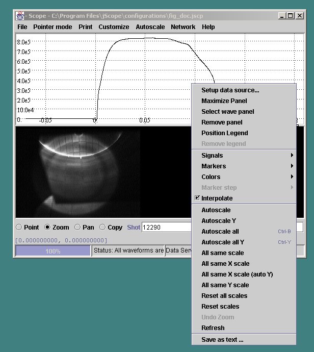
The item Setup data source... of this menu defines the contents of the selected panel and activates a setup form. The form is as follows

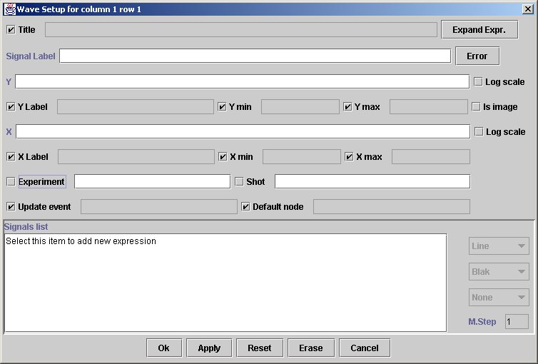
and defines the following fields:

• Title: the title of the panel (optional)
• Signal Label: the string to appear in the legend associated with the signal. If no label is defined, the definition of the Y axis of the signal is displayed.
• Y: the y axis of the signal. X and Y expression can be expanded by means of the Expand Expr. button.
• Y label: the label associated with y axis (optional).
• X: the x axis of the signal (optional, see below how jScope handles the case in which no x axis is specified)
• X label: the label associated with x axis (optional)
• Xmin, Xmax, Ymin, Ymax: maximum and minimum values for x and y axis (optional)
• Experiment: the name of the experiment (pulse file)
• Shot: the shot number
• Update event: the name of the event which generates an automatic update
• Default node: the default position used in the signal definition. The meaning of this optional information depends on the actual data server. In MdsDataServer it refers to the default node position in the tree-structured pulse file.

It is possible to define a set of signals using the form: after filling the fields and pressing <return>, the signal is added to the list. Definitions can be modified by selecting the signal on the list. To add a new signal to the list, select the first item; to remove a signal from the list, select it and press <del>.
Clicking the expand expr button, a popup window is displayed, which allows easier typing of long specifications of the X and Y axis. It is possible then to define maximum and minimum errors for displaying error bars, by clicking button error....  Most fields have a toggle button associated with them: when selected, the value of the corresponding field is taken from the global configuration (see before). For the definition of the shot field it is also possible to use the bottom shot field. In this case a set or a range of shots can be defined: a set is specified by the following syntax: [<sho1>, ,shot2>, ...]; a range by: <first_shot>:<last_shot>. Once a signal has been added to the list, the corresponding color and type of marker can be set first selecting the signal and then using the pull-down menus on the right of the form.
When a signal in the signal list is selected in the Setup data source popup form, it is possible to define the associated marker and color, as well to define whether the interpolating line has to be displayed and the marker step, i.e. the number of data points for each visible marker.

The Select Wave Panel item of the Waveform popup menu allows the selection of the associated waveform (indicated by a red border around the selected waveform). Waveform selection is used as a fast way for defining waveforms: in this case the name of the signal can be typed in the bottom Signal text field and inserted in the selected waveform by pressing <Return>. The name refers only to the Y Value field of the Setup popup form; all the other parameters are taken from the global configuration. Multiple waveforms can be inserted by consecutively typing the waveform name and pressing <Return> in the Signal field. If no wave panel is selected and new signals are entered, a new panel is created for each signal.

The other two items Position legend and Remove legend of the Waveform popup menu allow the definition of legend for the signals associated with the waveform. The legend can be activated/deactivated and positioned where needed in the waveform window. The associated labels associated with the signals are displayed in the legend. If no label is associated with a given signal, the Y-value name is displayed instead.

The Signals item of the Waveform popup menu allows a rapid activation/deactivation of the currently defined signals. It is useful when dealing with multiple signals to individually define their visibility in the waveform panel.

The Marker, Marker-step, Colors and Interpolate items of the Waveform popup menu are active only in point mode, i.e. when one signal is selected, and allow a rapid definition of the associated graphical configuration without opening the Setup data source popup form.

The other items of the popup list allow rescalings of waveforms, and their meanings are clear from the associated label.

Finally the last item Save as Text writes the displayed waveforms points in a text file, as described before..

jScope and Images

It is possible with jScope to look at sequences of frames (usually produced by a camera) and to correlate them with other waveforms. Using standard jdk, it is possible to look at gif, jpeg and bitmap images. It is also possible to look at other formats by installing the standard java extension JAI (Java Advanced Imaging).
A jScope panel can be connected to a sequence of frames by selecting the is_image check box in the data setup dialog. When image mode is selected, the fields of the setup data dialog are changed and looks like the following:

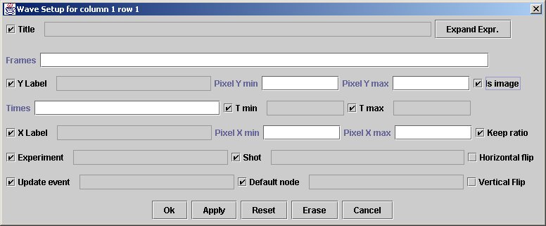
where the fields have the following meaning

• Title: title written above the image
• Frames: frame sequence name (the following section will explain how names are associated with frame sequences)
• Times: defines the time to be associated with each frame. If timing information is stored into the frame set, there is no need to fill this field. Otherwise it will refer to a vector of times.
• t min, t.max: defines minimum and maximum time to be considered in the frame sequence. NOTE: this field is very important for very large sequences of frames. jScope in fact discards frames whose time is outside the specified interval, thus freeing memory resources. The default value(as specified by the associated checkboxes) is taken from xmin and xmax fields of the global setting.
• Y label: the label associated with y axis (optional)
• X label: the label associated with x axis (optional)
• Pix Xmin, Pix Xmax, Pix Ymin, Pix Ymax: maximum and minimum values for the region of interest in the image(in pixel)
• Experiment: the name of the experiment (pulse file)
• Shot: the shot number
• Update event: the name of the event which generates an automatic update.
• Default node: the default position in the signal definition.
• Keep ratio: maintain original aspect ratio in image resizing.
• Flip horizontal, Flip vertical: optional image flip.

and the checkboxes indicate whether the corresponding value is taken from the global setup.
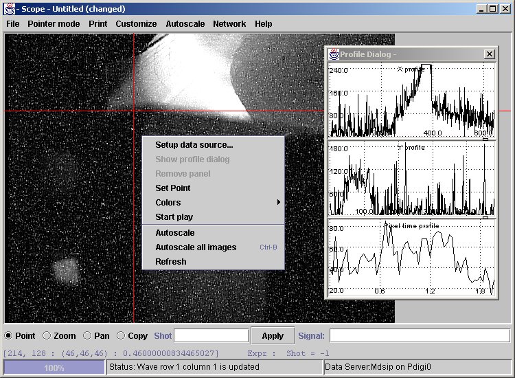
Once the frame sequence has been loaded, the first frame of the sequence is displayed. When in zoom mode, it is possible to enlarge portions of the image. When in point mode, the frame sequence is synchronized with the other displayed waveforms. This means that moving the cursor over a waveform will also update the displayed frame accordingly. When in point mode, <ctrl>MB1 click will proceed one frame further (moving in correspondence the cursor over the other waveforms). Conversely, <shift>MB1 click will go back one frame.
When a panel is displaying a frame sequence, the popup menu will look as follows:

where some frame-specific menu items are defined as follows(the others have the same meaning as when looking at waveforms):

• Start play: start frame animation. When in zoom mode, the cursor is moved over the other waveforms, and animation is performed in step for the other frame panels. During animation the item is changed to stop play for stopping the animation.
• Show profile dialog: enable a popup dialog showing X,Y and Z profiles centered at the selected point (when in point mode).
• Autoscale: used to come back to the original frame width after zooming.
• Autoscale all images: the same as above, performed on all the frame panels.

How to integrate frame sequences in jScope using MDSplus (MdsDataProvider)

When using a MDSplus data server (mdsip) for getting data in jScope, the following TDI functions must be provided for displaying frame sequences, and will be invoked by jScope in the given sequence:

• JavaGetAllFrames(in _experiment, in_frame_name, in_shot) : this TDI function receive the experiment (string), the shot (int) and the frame sequence name(string) as defined in the popup dialog. This fun will return 0 if frames are stored in separate items, thus making jScope separately request each frame of the request. Currently this fun will return a non zero value only for multiframe gif format implemented at CMOD. In this case, the content of the file is returned in the form of a byte array as it stands (it will be decoded by jScope) and the following funs are not called.
• JavaGetFrameTimes(in _experiment, in _frame_name, in _shot): this TDI function receives the same parameters of the above function, and will return an array of times, specifying the time associated with each frame.
• JavaGetFrameAt(in _experiment, in _frame_name, in _shot, in _frame_idx): this TDI function receives in addition the index of the required frame in the frame sequence. It will be called by jScope as many times as the dimension of the time vector returned by JavaGetFrameTimes, and will provide the selected image (frame) as it stands in the form of a byte array.

The property file of jScope
When started, jScope looks for the jScope.properties file. This file allows user configuration of jScope and may look as follows:

jScope.directory=N:\\Taliercio\\Applicazioni JAVA\\jScope\\config_scope
jScope.cache_directory=
jScope.cache_size=
jScope.reversed=false
jScope.grid_mode=Dotted
jScope.x_grid=5
jScope.y_grid=5
jScope.item_color_0=Blak,java.awt.Color[r=0,g=0,b=0]
jScope.item_color_1=Blue,java.awt.Color[r=0,g=0,b=255]
jScope.item_color_2=Cyan,java.awt.Color[r=0,g=255,b=255]
jScope.item_color_3=DarkGray,java.awt.Color[r=64,g=64,b=64]
jScope.item_color_4=Gray,java.awt.Color[r=128,g=128,b=128]
jScope.item_color_5=Green,java.awt.Color[r=0,g=255,b=0]
jScope.item_color_6=LightGray,java.awt.Color[r=192,g=192,b=192]
|jScope.item_color_7=Magenta,java.awt.Color[r=255,g=0,b=255]
jScope.item_color_8=Orange,java.awt.Color[r=255,g=200,b=0]
jScope.item_color_9=Pink,java.awt.Color[r=255,g=175,b=175]
jScope.item_color_10=Red,java.awt.Color[r=255,g=0,b=0]
jScope.item_color_11=Yellow,java.awt.Color[r=255,g=255,b=0]
jScope.default_server = 4
jScope.data_server_1.name = Jet MDSPlus data
jScope.data_server_1.class = JetMdsDataProvider
 jScope.data_server_2.name=TWU data
jScope.data_server_2.class=TwuDataProvider
jScope.data_server_2.browse_class=TextorBrowseSignals
jScope.data_server_2.browse_url=http://ipptwu.ipp.kfa-juelich.de/
jScope.data_server_3.name=Jet data
jScope.data_server_3.class=JetDataProvider
jScope.data_server_4.name = RFX data server
jScope.data_server_4.argument = 150.178.3.80
jScope.data_server_4.class=MdsDataProvider
jScope.data_server_4.browse_class=MdsPlusBrowseSignals
jScope.data_server_4.browse_url=http://pdigi9.igi.pd.cnr.it/wwwai/rfx_jscope.html
jScope.data_server_5 = Ftu data server
jScope.data_server_5.argument = 192.107.51.84:8100
jScope.data_server_5.class = FtuDataProvider
jScope.data_server_6.name = Local MdsPlus data
jScope.data_server_6.class = LocalDataProvider
jScope.data_server_7 = Demo
jScope.data_server_7.class = DemoDataProvider 
 
The selectable properties of jScope.properties are the following:

• jScope.directory  defines the default directory for storing and retrieving configurations.
• jScope.cache_directory defines the cache directory. If the property is not defined, cached data are saved in /home_dir/jScopeCache.
• jScope.cache_size defines the maximum cache size (default 16 MBytes)
• jScope.grid_mode defines the grid selection.
• jScope.x_grid defines the tentative number of x labels.
• jScope.y_grid defines the tentative number of y labels.
• jScope.item_color_n defines the nth color in the color palette
• jScope.reversed if true defines black background.
• jScope.vertical_offset defines the dimension of the border between the drawn waveforms and the top and bottom limits of the panel.
• jScope.vertical_offset defines the dimension of the border between the drawn waveforms and the left and right limits of the panel.
• jScope.http_proxy_host defines the proxy server to be used when using HTTP connections.
• jScope.http_proxy_port defines the port of the proxy server to be used when using HTTP connections.
• jScope.default_server defined as the index of the default server in the server list

The following properties define the data servers available in the jScope environment. The nth data server is defined by the following properties:

• jScope.data_server_n.name  defines the associated name which will be shown in the server list.
• jScope.data_server_n.class defines the Java class of the corresponding data server
• jScope.data_server_n.argument (optional) defines the argument passed to the data server after creation. For example in MdsDataServer the argument defines the ip address of the corresponding mdsip server.
• jScope.data_server_n.browse_class (optional) defines, if signal browsing enabled, the class of the browser which is activated by jScope when the file->browse signals item is selected.
• jScope.data_server_n.browse_url (optional) defines, if signal browsing enabled, the initial URL for the signal browser.

How to adapt jScope to a proprietary data acquisition system

Originally developed for MdsPlus, the architecture of jScope is now completely independent from a particular data system. This means that jScope can be adapted to every data system.

For a seamless integration of a new data system into the jScope framework, it suffices to develop the implementation of three Java interfaces. Once such implementations have been added to the jScope classes, and the declaration of the new data server has been added into the property file, the data server can be used to visualize signals and frame sequences with jScope. There is therefore no need of changing any line of code of the core jScope application.

The main interface is DataProvider, which defines a set of methods which need to be implemented. The other two interfaces, WaveData and FrameData, describe a signal and a frame sequence, respectively, as they are returned by the data access methods of DataProvider.

For a complete reference of the methods defined in these interfaces, and on how to implement them, refer to the javadoc description of DataProvider.

  For further information, you can contact jScope authors at the following e-mail address: manduchi@igi.pd.cnr.it

jScope related classes

  It is possible to use the plotting classes outside the jScope application. In particular it is possible to define applets for plotting signals, and to integrate plotting classes into other java C/C++ application.
The plotting capabilities are exported by the CompositeWaveDisplay class. Detailed information on how to use CompositeWaveDisplay class is provided here.